Scalability of Parallel Architectures

• A parallel architecture is said to be scalable if it can be expanded (reduced) to a larger (smaller) system with a linear increase (decrease) in its performance (cost). This general definition indicates the desirability for providing equal chance for scaling up a system for improved performance and for scaling down a system for greater cost-effectiveness and/or affordability.
• Scalability is used as a measure of the system's ability to provide increased performance, for example, speed as its size is increased. In other words, scalability is a reflection of the system's ability to efficiently utilize the increased processing resources.
• The scalability of a system can be manifested as in the forms; speed, efficiency, size, applications, generation, and heterogeneity.
• In terms of speed, a scalable system is capable of increasing its speed in proportion to the increase in the number of processors.
  • Consider, for example, the case of adding $m$ numbers on a 4-cube ($n=16$ processors) parallel system.
  • Assume for simplicity that $m$ is a multiple of $n$. Assume also that originally each processor has ($m=n$) numbers stored in its local memory. The addition can then proceed as follows.
    • First, each processor can add its own numbers sequentially in ($m=n$) steps. The addition operation is performed simultaneously in all processors.
    • Secondly, each pair of neighboring processors can communicate their results to one of them whereby the communicated result is added to the local result.
    • The second step can be repeated ($log_2 n$) times, until the final result of the addition process is stored in one of the processors.
    • Assuming that each computation and the communication takes one unit time then the time needed to perform the addition of these $m$ numbers is
      $$T_p=(m/n)+2*log_2 n$$

    • Recall that the time required to perform the same operation on a single processor is $T_s=m$. Therefore, the speedup is given by
      $$S=\frac{m}{(m/n)+2*log_2 n}$$

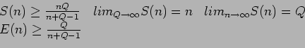
  • Figure 3.3a provides the speedup $S$ for different values of $m$ and $n$. It is interesting to notice from the table that for the same number of processors, $n$, a larger instance of the same problem, $m$, results in an increase in the speedup, $S$. This is a property of a scalable parallel system.

  Figure 3.3: The Possible Speedup and Efficiency for Different $m$ and $n$.

  

  
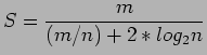
• In terms of efficiency, a parallel system is said to be scalable if its efficiency can be kept fixed as the number of processors is increased, provided that the problem size is also increased.
  • Consider, for example, the above problem of adding $m$ numbers on an n-cube. The efficiency of such a system is defined as the ratio between the actual speedup, $S$, and the ideal speedup, $n$.
    $$E=\frac{S}{n}=\frac{m}{m+2n*log_2 n}$$

  • Figure 3.3b shows the values of the efficiency, $E$, for different values of $m$ and $n$. The values in the table indicate that for the same number of processors, $n$, higher efficiency is achieved as the size of the problem, $m$, is increased.
  • However, as the number of processors, $n$, increases, the efficiency continues to decrease.
  • Given these two observations, it should be possible to keep the efficiency fixed by increasing simultaneously both the size of the problem, $m$, and the number of processors, $n$. This is a property of a scalable parallel system.
  • It should be noted that the degree of scalability of a parallel system is determined by the rate at which the problem size must increase with respect to $n$ in order to maintain a fixed efficiency as the number of processors increases.
    • For example, in a highly scalable parallel system the size of the problem needs to grow linearly with respect to $n$ to maintain a fixed efficiency.
    • However, in a poorly scalable system, the size of the problem needs to grow exponentially with respect to $n$ to maintain a fixed efficiency.
  • It is useful to indicate at the outset that typically an increase in the speedup of a parallel system (benefit), due to an increase in the number of processors, comes at the expense of a decrease in the efficiency (cost).
  • In order to study the actual behavior of speedup and efficiency, we need first to introduce a new parameter, called the average parallelism $Q$.
    • It is defined as the average number of processors that are busy during the execution of given parallel software (program), provided that an unbounded number of processors are available.
    • The average parallelism can equivalently be defined as the speedup achieved assuming the availability of an unbounded number of processors.
  • It has been shown that once $Q$ is determined, then the following bounds are attainable for the speedup and the efficiency on an n-processor system:

    $$\begin{array}{lcc} S(n) \geq \frac{nQ}{n+Q-1} & lim_{Q\righta... ...row \infty} S(n)=Q E(n) \geq \frac{Q}{n+Q-1} & & \end{array}$$ (3.9)

    
    

  • The above two bounds show that the sum of the attained fraction of the maximum possible speedup, $S(n)/Q$, and attained efficiency, must always exceed 1.
  • Notice also that, given a certain average parallelism, $Q$, the efficiency (cost) incurred to achieve a given speedup is given by
    $$E(n)\geq\frac{Q-S(n)}{Q-1}$$

  • It is therefore fair to say that the average parallelism of a parallel system, $Q$, determines the associated speedup versus efficiency tradeoff.
• Size scalability; measures the maximum number of processors a system can accommodate. For example, the size scalability of the IBM SP2 is 512, while that of the symmetric multiprocessor (SMP) is 64.
• Application scalability; refers to the ability of running application software with improved performance on a scaled-up version of the system.
  • Consider, for example, an n-processor system used as a database server, which can handle 10,000 transactions per second. This system is said to possess application scalability if the number of transactions can be increased to 20,000 using double the number of processors.
• Generation scalability; refers to the ability of a system to scale up by using nextgeneration (fast) components.
  • The most obvious example for generation scalability is the IBM PCs. A user can upgrade his/her system (hardware or software) while being able to run their code generated on their existing system without change on the upgraded one.
• Heterogeneous scalability; refers to the ability of a system to scale up by using hardware and software components supplied by different vendors.
  • For example, under the IBM Parallel Operating Environment (POE) a parallel program can run without change on any network of RS6000 nodes; each can be a low-end PowerPC or a high-end SP2 node.
• In his vision on the scalability of parallel systems, Gordon Bell has indicated that in order for a parallel system to survive, it has to satisfy five requirements. These are size scalability, generation scalability, space scalability, compatibility, and competitiveness. As can be seen, three of these long-term survivability requirements have to do with different forms of scalability.
• As can be seen, scalability, regardless of its form, is a desirable feature of any parallel system. This is because it guarantees that with sufficient parallelism in a program, the performance, for example, speedup, can be improved by including additional hardware resources without requiring program change.
• Owing to its importance, there has been an evolving design trend, called design for scalability (DFS), which promotes the use of scalability as a major design objective. Two different approaches have evolved as DFS. These are overdesign and backward compatibility.
  • Using the first approach, systems are designed with additional features in anticipation for future system scale-up. An illustrative example for such approach is the design of modern processors with 64-bit address,that is, $2^{64}$ bytes address space. Assume that the current UNIX operating system supports only 32-bit address space. With memory space overdesign, future transition to 64-bit UNIX can be performed with minimum system changes.
  • The other form of DFS is the backward compatibility. This approach considers the requirements for scaled-down systems. Backward compatibility allows scaled-up components (hardware or software) to be usable with both the original and the scaled-down systems. As an example, a new processor should be able to execute code generated by old processors. Similarly, a new version of an operating system should preserve all useful functionality of its predecessor such that application software that runs under the old version must be able to run on the new version.