Approximation of Functions with MATLAB I

1. Write a MATLAB program to generate Chebyshev polynomials. (Hint: Use the M-file given in the book.)
   Solution:

   function T=Tch(n)
   if n==0
   	disp('1')
   elseif n==1
   	disp('x')
   else
   	t0='1';
   	t1='x';
   	for i=2:n
   		T=symop('2*x','*',t1,'-',t0);
   		t0=t1;
   		t1=T;
   	end 
   end
   

   save with the name Tch.m. Then;

   >>Tch(5)
   ans =2*x*(2*x*(2*x*(2*x^2-1)-x)-2*x^2+1)-2*x*(2*x^2-1)+x
   >>collect(ans)
   ans= 16*x^5-20*x^3+5*x
   

   For Matlab7 users,

   function s = symop(varargin);
   %SYMOP Obsolete Symbolic Toolbox function.
   % SYMOP takes any number of arguments, including  %'+','-','*','/','^',
   % '(' and ')', concatenates them and symbolically evaluates the %result.
   % Copyright (c) 1993-98 by The MathWorks, Inc.
   % $Revision: 1.2 $ $Date: 1997/11/29 01:06:41 $
   s = [];
   for k = 1:nargin
      v = varargin{k};
      if ~ischar(v), v = char(sym(v)); end
      switch v
      case {'+','-','*','/','^','(',')'}
         s = [s v];
      otherwise
         s = [s 'sym(''' v ''')'];
      end
   end
   s = eval(s);
   

2. Write a MATLAB program using Chebyshev polynomials to economize a Maclaurin series for $e^x$ in the interval [0,1] with a precision of $0.0001$. Tabulate the error values. (Hint: Utilize the M-file given in the book.) Solution:

   >> syms x
   >> ts=taylor(exp(x),8)
   ts =1+x+1/2*x^2+1/6*x^3+1/24*x^4+1/120*x^5+1/720*x^6+1/5040*x^7
   >> cs=collect(Tch(7))
   cs = 64*x^7-112*x^5+56*x^3-7*x
   >> es=ts-cs/factorial(7)/2^6
   es =
   1+46081/46080*x+1/2*x^2+959/5760*x^3+1/24*x^4+5/576*x^5+1/720*x^6
   >> vpa(es,7)
   ans = 1.+1.000022*x+.5000000*x^2+.1664931*x^3+.4166667e-1*x^4
   +.8680556e-2*x^5+.1388889e-2*x^6
   

3. The Chebyshev series and Maclaurin series for $e^x$ are given as the following;
   $$\begin{array}{l} e^x=0.9946+0.9973x+0.5430x^2+0.1772x^3 \\ e^x=1+x+0.5x^2+0.1667x^3\\ \end{array}$$
   • Tabulate the error values for the interval [-1,1].
   • Plot the error values for the interval.
   Solution:
   

   function week8lsgitem3(ll,ul,s)
   format short;
   %format long;
   disp('     x        e^x    Chebyshev   Error   Maclaurin   Error')
   x =(ll:s:ul)';
   taylor=exp(x);
   max=(ul-ll)/s+1;
   for i=1:max
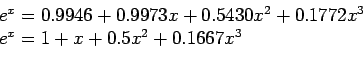
   chebyshev=(0.9946 + 0.9973*x(i) + 0.5430*x(i)^2 + 0.1772*x(i)^3);
   errorchebyshev(i)=taylor(i)-chebyshev;
   maclaurin=(1+x(i)+0.5*x(i)^2+0.1667*x(i)^3);
   errormaclaurin(i)=taylor(i)- maclaurin;
   D=[x(i),taylor(i),chebyshev,errorchebyshev(i),maclaurin,errormaclaurin(i)];  
   disp(D); 
   end 
   plot(x,errorchebyshev,'o',x,errormaclaurin,'-')
   

   save with the name week8lsgitem3.m. Then;

   >> week8lsgitem3(-1,1,0.1)
        x        e^x    Chebyshev   Error   Maclaurin   Error
      -1.0000    0.3679    0.3631    0.0048    0.3333    0.0346
   
      -0.9000    0.4066    0.4077   -0.0011    0.3835    0.0231
   
      -0.8000    0.4493    0.4536   -0.0042    0.4346    0.0147
   
      -0.7000    0.4966    0.5018   -0.0052    0.4878    0.0088
   
      -0.6000    0.5488    0.5534   -0.0046    0.5440    0.0048
   
      -0.5000    0.6065    0.6096   -0.0030    0.6042    0.0024
   
      -0.4000    0.6703    0.6712   -0.0009    0.6693    0.0010
   
      -0.3000    0.7408    0.7395    0.0013    0.7405    0.0003
   
      -0.2000    0.8187    0.8154    0.0033    0.8187    0.0001
   
      -0.1000    0.9048    0.9001    0.0047    0.9048    0.0000
   
            0    1.0000    0.9946    0.0054    1.0000         0
   
       0.1000    1.1052    1.0999    0.0052    1.1052    0.0000
   
       0.2000    1.2214    1.2172    0.0042    1.2213    0.0001
   
       0.3000    1.3499    1.3474    0.0024    1.3495    0.0004
   
       0.4000    1.4918    1.4917    0.0001    1.4907    0.0012
   
       0.5000    1.6487    1.6511   -0.0024    1.6458    0.0029
   
       0.6000    1.8221    1.8267   -0.0046    1.8160    0.0061
   
       0.7000    2.0138    2.0196   -0.0058    2.0022    0.0116
   
       0.8000    2.2255    2.2307   -0.0051    2.2054    0.0202
   
       0.9000    2.4596    2.4612   -0.0016    2.4265    0.0331
   
       1.0000    2.7183    2.7121    0.0062    2.6667    0.0516
   

   Figure 6.3: plot(x,errorchebyshev,'o',x,errormaclaurin,'-').