Next: About this document ...
| iteration | |||
| 1 | 0.50000000000000 | 0.33333333333333 | 0.50000000000000 |
| 2 | 0.25000000000000 | 0.36017071357763 | 0.35491389049015 |
| 3 | 0.37500000000000 | 0.36042168047602 | 0.36046467792776 |
| 4 | 0.31250000000000 | 0.36042170296032 | 0.36042169766326 |
| 5 | 0.34375000000000 | 0.36042170296032 | 0.36042170296032 |
| iteration | |||
| 1 | 3.3070e-01 | -1.0000e+00 | 3.3070e-01 |
| 2 | -2.8662e-01 | -6.8418e-02 | -1.3807e-02 |
| 3 | 3.6281e-02 | -6.2799e-04 | 1.0751e-04 |
| 4 | -1.2190e-01 | -5.6252e-08 | -1.3252e-08 |
| 5 | -4.1956e-02 | -6.6613e-16 | 2.2204e-16 |
| iteration | |
||
| 1 | |||
| 2 | |||
| 3 | |||
| 4 | |||
| 5 |
|
|
|
|
| iteration | |
||
| 1 | 1.3958e-01 | -2.7088e-02 | 1.3958e-01 |
| 2 | -1.1042e-01 | -2.5099e-04 | -5.5078e-03 |
| 3 | 1.4578e-02 | -2.2484e-08 | 4.2975e-05 |
| 4 | -4.7922e-02 | -1.6653e-16 | -5.2971e-09 |
| 5 | -1.6672e-02 | 1.1102e-16 | 2.2204e-16 |
|
|
|
|
| 7.1644e+00 | -3.6916e+01 | 7.1644e+00 |
| -1.2640e+00 | 1.0793e+02 | -2.5342e+01 |
| -7.5744e+00 | 1.1163e+04 | -1.2816e+02 |
| -3.0421e-01 | 1.3501e+08 | -8.1130e+03 |
| 2.8744e+00 | -1.5000e+00 | -2.3856e+07 |
First method does not converge, while the second method converges faster than the third one. The second method converges at the fourth step because the next step is also at the same error level and they are small enough. The third one seems to converge at the fifth step since it is small enough.
From the error ratio table, first method has a monotonic behavior and it is also seen that it does not converge. The second method is the fastest method and it approaches to the exact value with the square of the error of the previous step in each iteration. The third one is also fast method but with the same ratio of the previous step.
| |
|||
| Name |
| |
|||
| Name | Bisection | Newton | Muller |
Since we do not care about the prices for each method, dealing just
with the numbers. Newton's method is the best one since it converges quadratically, so it is the fastest one.
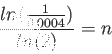
>>solve('2*x-6*log(x)')
ans =
    -3*lambertw(-1/3)
 -3*lambertw(-1,-1/3)
>> -3*lambertw(-1/3)
ans =    1.8572
>>  -3*lambertw(-1,-1/3)
ans =    4.5364
write the function
function fx=func(x)
fx=2*x-6*log(x);
save as func.m
write the function
function fx=funcdiff(x)
fx=2-6/x;
save as funcdiff.m
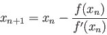
>> format long
>> x0=1.5;x1=x0-(func(x0)/funcdiff(x0))
x1 =   1.78360467567551
>> x2=x1-(func(x1)/funcdiff(x1))
x2 =   1.85354064971539
>> x3=x2-(func(x2)/funcdiff(x2))
x3 =   1.85717450334217
>> x4=x3-(func(x3)/funcdiff(x3))
x4 =   1.85718386014596
>> x5=x4-(func(x4)/funcdiff(x4))
x5 =   1.85718386020784
>> x6=x5-(func(x5)/funcdiff(x5))
x6 =   1.85718386020784
>> x7=x6-(func(x6)/funcdiff(x6))
x7 =   1.85718386020784
or start with
>> x0=3.1;x1=x0-(func(x0)/funcdiff(x0))
x1 =  12.22039636867234
>> x2=x1-(func(x1)/funcdiff(x1))
x2 =   5.97649660388231
>> x3=x2-(func(x2)/funcdiff(x2))
x3 =   4.74567026655091
>> x4=x3-(func(x3)/funcdiff(x3))
x4 =   4.54457398303521
>> x5=x4-(func(x4)/funcdiff(x4))
x5 =   4.53641793698142
>> x6=x5-(func(x5)/funcdiff(x5))
x6 =   4.53640365501743
>> x7=x6-(func(x6)/funcdiff(x6))
x7 =   4.53640365497353
>> x8=x7-(func(x7)/funcdiff(x7))
x8 =   4.53640365497353
>> x9=x8-(func(x8)/funcdiff(x8))
x9 =   4.53640365497353
same result.
![\begin{displaymath}
\left[
\begin{array}{rrrr}
1 &-2 &4&6\\
8 &-3 &2&2\\
-1 &10 &2&4\\
\end{array} \right]
\end{displaymath}](img35.png)
 %**********************************************
 %i) Ax=b
 >> A=[1 -2 4; 8 -3 2; -1 10 2]
 >> b=[6 2 4]
 >> GEPivShow(A,b')
 Begin forward elimination with Augmented system:
      1    -2     4     6
      8    -3     2     2
     -1    10     2     4
 Swap rows 1 and 2;  new pivot = 8
 After elimination in column 1 with pivot = 8.000000
     8.0000   -3.0000    2.0000    2.0000
          0   -1.6250    3.7500    5.7500
          0    9.6250    2.2500    4.2500
 Swap rows 2 and 3;  new pivot = 9.625
 After elimination in column 2 with pivot = 9.625000
     8.0000   -3.0000    2.0000    2.0000
          0    9.6250    2.2500    4.2500
          0         0    4.1299    6.4675
 ans =   -0.1132     0.0755     1.5660 %these are x1, x2, x3
 >> det(A)
 ans =   318
 >> 8.0000*9.6250 *4.1299 %product of the diagonal of U
 ans =  318.0023
 % For LU-decomposition
 >> [L,U,pv] = luPiv(A)
 L =    1.0000         0         0
         -0.1250    1.0000         0
          0.1250   -0.1688    1.0000
 U =   8.0000   -3.0000    2.0000
          0    9.6250    2.2500
          0         0    4.1299
 pv =
      2
      3
      1
 % two times pivoting
 %**********************************************
 % ii) for not pivoting case;
 >> GEshow(A,b')
 Begin forward elimination with Augmented system:
      1    -2     4     6
      8    -3     2     2
     -1    10     2     4
 After elimination in column 1 with pivot = 1.000000
      1    -2     4     6
      0    13   -30   -46
      0     8     6    10
 After elimination in column 2 with pivot = 13.000000
     1.0000   -2.0000    4.0000    6.0000
          0   13.0000  -30.0000  -46.0000
          0         0   24.4615   38.3077
 ans =    -0.1132     0.0755    1.5660
 >> 1.0000*13.0000*24.4615
 ans =   317.9995
 % Solutions are the same. They are same because the system is
 % not ill-conditioned.
 %**********************************************
 % iii) LUx=bb now bb=[-3 7 -2]
 % First Check!
 % L an U is found above. Coution: b --> Permutted b
 % b=[2 4 6]
 % Ly=b : Find y
 >> y=GEPivShow(L,b')
 Begin forward elmination with Augmented system:
    1.000000000000000                   0                   0   2.000000000000000
   -0.125000000000000   1.000000000000000                   0   4.000000000000000
    0.125000000000000  -0.168831168831169   1.000000000000000   6.000000000000000
 After elimination in column 1 with pivot = 1.000000
    1.000000000000000                   0                   0   2.000000000000000
                    0   1.000000000000000                   0   4.250000000000000
                    0  -0.168831168831169   1.000000000000000   5.750000000000000
 After elimination in column 2 with pivot = 1.000000
    1.000000000000000                   0                   0   2.000000000000000
                    0   1.000000000000000                   0   4.250000000000000
                    0                   0   1.000000000000000   6.467532467532467
 y =
    2.000000000000000
    4.250000000000000
    6.467532467532467
 % Ux=y : Find x
 >> xx=GEPivShow(U,y)
 Begin forward elmination with Augmented system:
    8.000000000000000  -3.000000000000000   2.000000000000000   2.000000000000000
                    0   9.625000000000000   2.250000000000000   4.250000000000000
                    0                   0   4.129870129870130   6.467532467532467
 After elimination in column 1 with pivot = 8.000000
    8.000000000000000  -3.000000000000000   2.000000000000000   2.000000000000000
                    0   9.625000000000000   2.250000000000000   4.250000000000000
                    0                   0   4.129870129870130   6.467532467532467
 After elimination in column 2 with pivot = 9.625000
    8.000000000000000  -3.000000000000000   2.000000000000000   2.000000000000000
                    0   9.625000000000000   2.250000000000000   4.250000000000000
                    0                   0   4.129870129870130   6.467532467532467
 xx =
   -0.113207547169811
    0.075471698113208
    1.566037735849056
 % Same as before as expected!
 % Now for bb=[-3 7 -2]
 >> bb=[-3 7 -2]
 bb =    -3     7    -2
>> y=GEPivShow(L,bb')
Begin forward elmination with Augmented system:
   1.000000000000000                   0                   0  -3.000000000000000
  -0.125000000000000   1.000000000000000                   0   7.000000000000000
   0.125000000000000  -0.168831168831169   1.000000000000000  -2.000000000000000
After elimination in column 1 with pivot = 1.000000
   1.000000000000000                   0                   0  -3.000000000000000
                   0   1.000000000000000                   0   6.625000000000000
                   0  -0.168831168831169   1.000000000000000  -1.625000000000000
After elimination in column 2 with pivot = 1.000000
   1.000000000000000                   0                   0  -3.000000000000000
                   0   1.000000000000000                   0   6.625000000000000
                   0                   0   1.000000000000000  -0.506493506493507
y =
  -3.000000000000000
   6.625000000000000
  -0.506493506493507
>> xx=GEPivShow(U,y)
Begin forward elmination with Augmented system:
   8.000000000000000  -3.000000000000000   2.000000000000000  -3.000000000000000
                   0   9.625000000000000   2.250000000000000   6.625000000000000
                   0                   0   4.129870129870130  -0.506493506493507
After elimination in column 1 with pivot = 8.000000
   8.000000000000000  -3.000000000000000   2.000000000000000  -3.000000000000000
                   0   9.625000000000000   2.250000000000000   6.625000000000000
                   0                   0   4.129870129870130  -0.506493506493507
After elimination in column 2 with pivot = 9.625000
   8.000000000000000  -3.000000000000000   2.000000000000000  -3.000000000000000
                   0   9.625000000000000   2.250000000000000   6.625000000000000
                   0                   0   4.129870129870130  -0.506493506493507
xx =
  -0.075471698113208
   0.716981132075472
  -0.122641509433962
 % solution is completed
 %**********************************************
%**********************************************
%Switching rows 2 &3 first
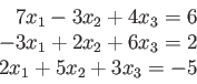
>> A=[7 -3 4; 2 5 3; -3 2 6]
>> B=[6 -5 2]
>> jacobi(A,B',P',0.01,20)
k = 1 P =
0.857142857142857
-1.000000000000000
0.333333333333333
k = 2 P =
0.238095238095238
-1.542857142857143
1.095238095238095
k = 3 P =
-0.429931972789116
-1.752380952380953
0.966666666666667
k = 4 P =
-0.446258503401361
-1.408027210884354
0.702494331065760
k = 5 P =
-0.147722708130871
-1.242993197278911
0.579546485260771
k = 6 P =
-0.006737933268545
-1.288638807904114
0.673803045027535
k = 7 P =
-0.080161229117497
-1.401586653709102
0.759510636000432
k = 8 P =
-0.177543215018434
-1.423641889953260
0.760448270010952
k = 9 P =
-0.187531249986227
-1.385251675999198
0.719109022475203
k = 10 P =
-0.147455873985486
-1.356452913490631
0.701318267006619
k = 11 P =
-0.124947401214053
-1.361808610609777
0.711756367504134
k = 12 P =
-0.133207328835124
-1.377074860016859
0.724795836262899
k = 13 P =
-0.147201132157454
-1.381594570223690
0.725754622254725
k = 14 P =
-0.149686028527138
-1.376572320489853
0.720264290662503
k = 15 P =
-0.144396303445653
-1.372284162986646
0.717347759233048
k = 16 P =
-0.140891932270305
-1.372650134161568
0.718563235939389
k = 17 P =
-0.141743335177466
-1.374781168655511
0.720437411918703
k = 18 P =
-0.143727593377335
-1.375565113080236
0.720722055296438
k = 19 P =
-0.144226222918065
-1.374942195826928
0.719991241004744
>> gseid(A,B',P',0.001,20)
k = 1 P =
0.857142857142857
-1.342857142857143
1.209523809523809
k = 2 P =
-0.409523809523810
-1.561904761904762
0.649206349206349
k = 3 P =
-0.183219954648526
-1.316235827664399
0.680468631897203
k = 4 P =
-0.095797430083144
-1.369962207105064
0.742088687326783
k = 5 P =
-0.154034481517475
-1.383639419789080
0.717529232504289
k = 6 P =
-0.145862169912057
-1.372172671537751
0.717793138889889
k = 7 P =
-0.141098652881830
-1.374236422181201
0.720862814286152
k = 8 P =
-0.143737217669745
-1.375022801503793
0.719805658333059
k = 9 P =
-0.143470148263374
-1.374495335694486
0.719763371099808
% Gauss-Seidel iterates much faster
![\includegraphics[scale=0.3]{numerical/26a.ps}](img19.png)