Newton's Method

Figure 3.6: Graphical illustration of the Newton's Method.

• One of the most widely used methods of solving equations is Newton's method.
• Like the previous ones, this method is also based on a linear approximation of the function, but does so using a tangent to the curve (see Figure).

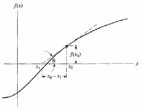
• Starting from a single initial estimate, $x_0$, that is not too far from a root, we move along the tangent to its intersection with the x-axis, and take that as the next approximation.
• This is continued until either the successive x-values are sufficiently close or the value of the function is sufficiently near zero.

• The calculation scheme follows immediately from the right triangle shown in Figure.
  $$tan\theta=f^{'}(x_0)=\frac{f(x_0)}{x_0-x_1}\Rightarrow x_1=x_0-\frac{f(x_0)}{f^{'}(x_0)}$$
  and the general term is:
  $$\boxed{x_{n+1}=x_{n}-\frac{f(x_n)}{f^{'}(x_n)},~n=0,1,2,\ldots}$$

• Newton's algorithm is widely used because, it is more rapidly convergent than any of the methods discussed so far. Quadratically convergent
• The error of each step approaches a constant K times the square of the error of the previous step.

• The number of decimal places of accuracy nearly doubles at each iteration.
• There is the need for two functions evaluations at each step, $f(x_n)$ and $f'(x_n)$ and we must obtain the derivative function at the start.
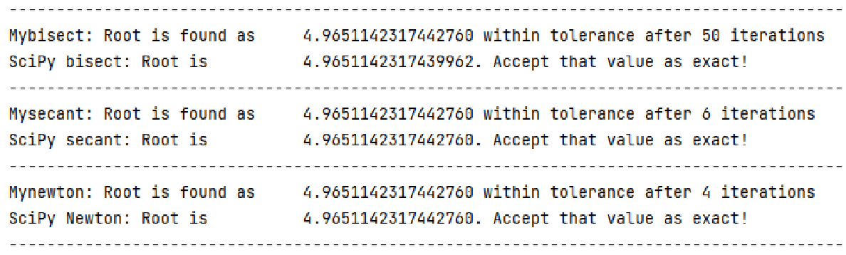
• If a difficult problem requires many iterations to converge, the number of function evaluations with Newton's method may be many more than with linear iteration methods. Because Newton's method always uses two per iteration whereas the others take only one.
• The method may converge to a root different from the expected one or diverge if the starting value is not close enough to the root.

• Apply Newton's method to $f(x)=3x + sin(x) - e^x$. (Example py-file: mynewton.py)
• Table shows the results from Newton's method for the same function that was used to illustrate bisection and secant methods.

Table 3.2: Newton's method for $f(x)=3x + sin(x) - e^x$, starting from $x_0=0$, using a tolerance value of 1E-16.

(Example py-file: blackbodyradiation.py)