Next: Simple Pendulum Up: Numerical Differentiation and Integration Previous: Variable force in one Contents
 .
.

 starting from an initial value.
.
approaches zero.
starting from an initial value.
.
approaches zero.

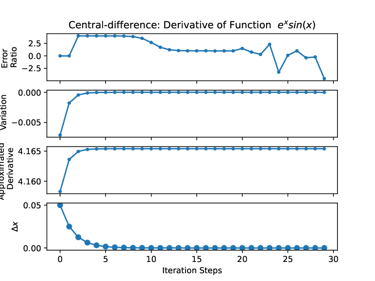
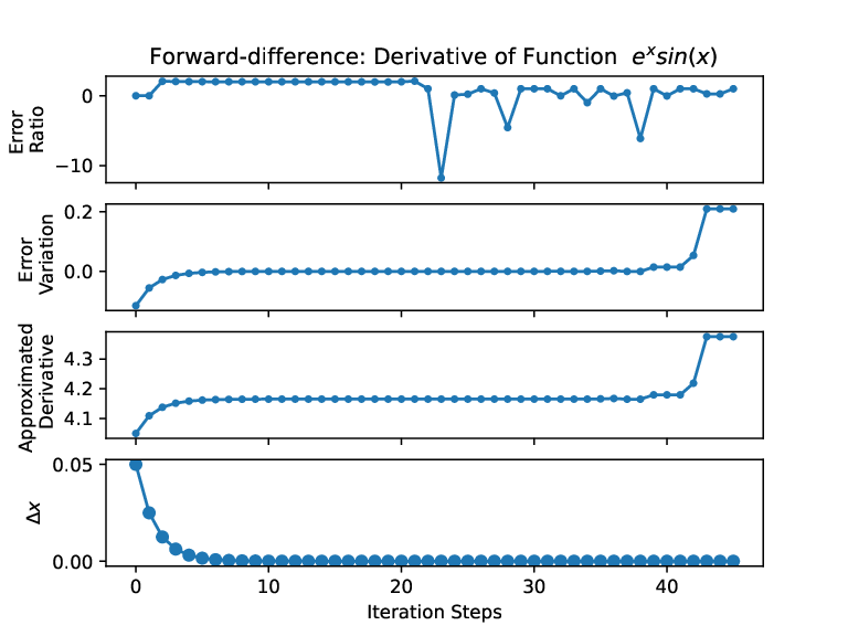
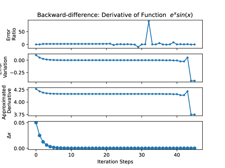
 . The analytical answer is 4.1653826.
Apply Forward-difference approximation to
 . (Example py-file:
myforwardderivative.py)
. (Example py-file:
myforwardderivative.py)
 and halving each time. Table gives the results.
is reduced until about
and halving each time. Table gives the results.
is reduced until about
 .
is halved until gets quite small, at which time round off affects the ratio.
smaller than
.
is halved until gets quite small, at which time round off affects the ratio.
smaller than
 , the error of the approximation increases due to round off.
is when the effects of round-off and truncation errors are balanced.
, the error of the approximation increases due to round off.
is when the effects of round-off and truncation errors are balanced.
 . (Example py-file:
mybackwardderivative.py)
. (Example py-file:
mybackwardderivative.py)
 for :
for :

 is at some point between and
  .
.
 , we get
 , it turns out that
 is between and
  .
.
 .
.
 |
 terms cancel.
 . (Example py-file:
mycentralderivative.py)
. (Example py-file:
mycentralderivative.py)
![\begin{table}\begin{center}
\includegraphics[scale=0.3]{images/5-1a}
\end{center}
\end{table}](img124.svg)
![\begin{table}\begin{center}
\includegraphics[scale=0.3]{images/5-1b}
\end{center}
\end{table}](img129.svg)


![\begin{table}\begin{center}
\includegraphics[scale=0.3]{images/5-1c}
\end{center}
\end{table}](img143.svg)