Trial-and-Error (Linear Shooting) Method

Figure 5.5: First guess.

Figure 5.6: Second guess.

...

Figure 5.7: Expected result.

• The basic approach in solving boundary value and eigenvalue problems is known as the trial-and-error method.
  • At one boundary, the solution is started by giving an estimated value to the missing initial condition,
  • A trial solution is then found with either Euler or Runge-Kutta method at the other boundary (First guess),
  • How much deviation from the given boundary condition is determined,
  • Taking this deviation into account, a new solution is restarted with a new estimation (Second guess),
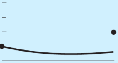
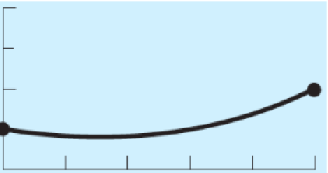
  • This process is repeated ($\ldots$) until the other boundary condition is satisfied (Expected result).

• Let's see this method on an example:

  	$$y''(x)-(4x^2-2)y$$	$$= 0$$	$$y(0)$$	$$=1.0 \nonumber$$
  		$$with~BCs$$	$$y(1)$$	$$=1/e=0.36787944 \nonumber$$

• This differential equation has the solution of $y=e^{(-x^2)}$ (Gaussian function).

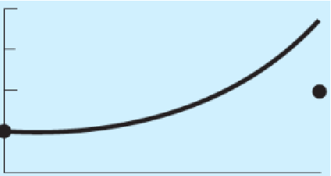
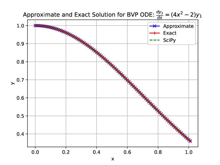
First, let's transform this boundary value problem into a first-order system of equations:

• $y_1=y$
• $y_2=y'$
• $\frac{dy_1}{dx}= y_2$
• $\frac{dy_2}{dx}=(4x^2-2)y_1$

• Notice that the boundary conditions are given only for
  $y_1$: $y_1(0)=1.0$ and $y_1(1)=0.368$.
• Notice that there is no initial condition for $y_2$.
• Now, we have a set of equations.

• Here, let's take an estimated initial value of $a$:

  $$\textbf{first~guess}:~ y_2(0)=a$$

• Now, find the solutions $y_1(x)$ and $y_2(x)$ (by let's say RK4) with these $y_1(0)$ and $y_2(0)$ values.
• Denote the value obtained for $y_1$ in the other boundary with $y_{1a}(1)$
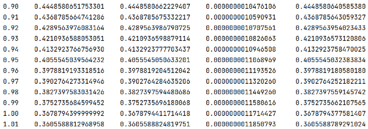
• and find the difference ($\Delta_a$) with the real one $y_1(1)$ (here, 0.368):

  $$y_2(0)=a \rightarrow solution:~ y_{1a}(x) \rightarrow \Delta_a=y_{1a}(1)-y_1(1)$$

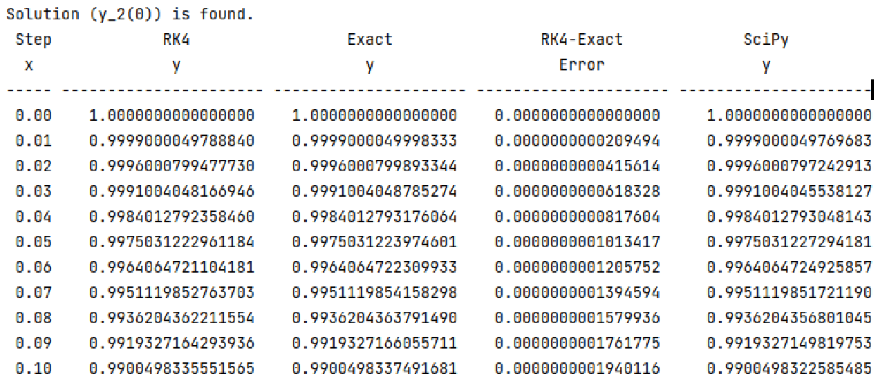
• Now, let's make a second (another) guess of $b$ and calculate the error again at the other boundary:

  $$y_2(0)=b \rightarrow solution:~ y_{1b}(x) \rightarrow \Delta_b=y_{1b}(1)-y_1(1)$$

• Remind the secant methods for root finding.
• After these two estimated shoots, the most accurate starting value to choose will be the extension of the line passing through two points:

  $$y_2(0)=b-\dfrac{\Delta_b}{\Delta_b-\Delta_a}(b-a)$$

• Then, the calculation (RK4) is repeated with this selected value by secant method.
• Finally, the solution is found when the margin of error in the other boundary is smaller than a certain tolerance.
• (Example py-file: mylinearshooting.py)

Figure 5.8: Solution for the Boundary Value Problem for the ODE: $y''(x)-(4x^2-2)y=0$.

Figure 5.9: Solution for the Boundary Value Problem for the ODE: $y''(x)-(4x^2-2)y=0$.