Hydrogen Atom

• In quantum mechanics, the hydrogen atom is considered as a system of electrons with a charge of $-e$ around a proton with a charge of $+e$.
• If the electrostatic potential energy between the electron-proton is substituted in the Schrödinger equation as $V(r)=-e^2/r$,

  $$-\frac{\hbar^2}{2m_r}\nabla^2\psi(\vec{r})-\frac{e^2}{r}\psi(\vec{r})=E\psi( \vec{r})$$

  Here $m_r=m_em_p/(m_e+m_p)$ is the reduced mass of the electron-proton system.
• Since the potential energy depends only on the distance $r$, the solution is defined with the spherical coordinates $(r, \theta, \phi)$ in three-dimensional space:

  $$\psi(r,\theta,\phi)=R(r)Y(\theta,\phi)$$

• The solutions of the equation provided by the angular variables $(\theta,\phi)$ are independent of the $V(r)$ potential and consist of functions called spherical harmonics $Y(\theta,\phi)$.
• The equation provided by the $R(r)$ function is called radial Schrödinger equation.

  $$-\frac{\hbar^2}{2m_r}\left[ \frac{d^2R}{dr^2}+\frac{2}{r} \frac{d... ...ft [\frac{l(l+1)\hbar^2}{2m_rr^2}-\frac{e^2}{r} \right] R(r)=-\vert E\vert R(r)$$

• Attempt to find the bound energy (eigen)values and wave (eigen)functions of the radial Schrödinger equation numerically :
• First, it is necessary to make the radial equation dimensionless bu defining a new wavefunction:

  $$u(r)=rR(r)$$

• The radial equation in terms of this new function $u(r)$ becomes simpler:

  $$\frac{d^2u}{dr^2}- \left[\frac{l(l+1)}{r^2}-\frac{2m_re^2}{\hbar^2 r} \right]u (r)=-\frac{2m_r\vert E\vert}{\hbar^2}u(r)$$

• Now, a variable change is made as the following:

  $k=\frac{\sqrt{2m_r\vert E\vert}}{\hbar}$,

  $\rho=2kr$,

  $\lambda^2=\frac{1}{ka_0}=\frac{\Re }{\vert E\vert}$

  Here, the Rydberg constant $\Re$ and the Bohr radius $a_0$ are defined as:

  $a_0=\frac{\hbar^2}{m_re^2}$,

  $\Re=\frac{\hbar^2}{2m_ra_0^2}$

• As a result of these changes, the dimensionless radial equation becomes:

  $$\boxed{\frac{d^2u}{d\rho^2}-\frac{l(l+1)}{\rho^2}u+\left( \frac{\lambda}{\rho}-\frac{1 }{4} \right) u=0}$$ (5.5)

  where l is orbital quantum number and $\lambda$ is principal quantum number.

Numerical Solution. Firstly, transform this quadratic Equation 5.5 into a system of linear (first degree) equations:

$$u \rightarrow y_1$$

$$\frac{du}{d\rho} \rightarrow y_2$$

with these values ( $y_1~ and~y_2$), the system of equations to be solved: (Now, we have a set of equations.)

	$$\frac{dy_1}{d\rho}$$	$$=y_2$$
	$$\frac{dy_2}{d\rho}$$	$$=\left[ \frac{l(l+1)}{\rho^2} -\left( \frac{\lambda}{\rho}-\frac{1} {4}\right) \right] y_1$$

• For the initial conditions:
  • $u(0) \sim 0$
  • Since the absolute magnitude of the wave function has no physical meaning, the arbitrary value $u'(0)=1$ can be taken.
• Then;

  $y_1(0)=0$

  and   $y_2(0)=1$

(Example py-file: Program that solves the radial Schrödinger equation for the hydrogen atom: hydrogenatom.py)

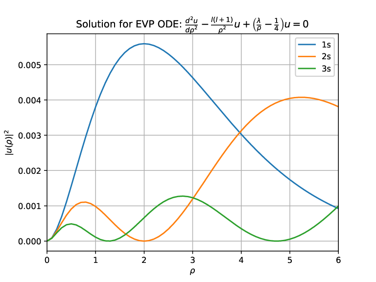
• Program does not graph the $u(r)$ functions, but the $\vert u\vert^2$ probability densities, which is physically meaningful.
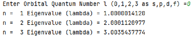
• It calculates according to the $l$ quantum number which is supplied by the user.
• The error margin is to be increased by increasing $n$ quantum number.

Figure 5.14: Solution for the Eigenvalue Problem for the ODE: $\frac {dy_2}{d\rho }=\left [ \frac {l(l+1)}{\rho ^2} -\left ( \frac {\lambda }{\rho }-\frac {1} {4}\right ) \right ] y_1$.

Figure 5.15: Solution for the Eigenvalue Problem for the ODE: $\frac {dy_2}{d\rho }=\left [ \frac {l(l+1)}{\rho ^2} -\left ( \frac {\lambda }{\rho }-\frac {1} {4}\right ) \right ] y_1$.