Hands-on-Interpolation and Curve Fitting with MATLAB III

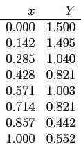
1. Fitting a cubic to the data by using MATLAB. For the given data points;
   $$\begin{array}{rr} x & Y \hline 0.000 & 1.500 \\ 0.142 &... ...714 & 0.821 \\ 0.857 & 0.442 \\ 1.000 & 0.552 \\ \end{array}$$
   • Evaluate the cubic on the $x$ data and plot

     
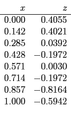
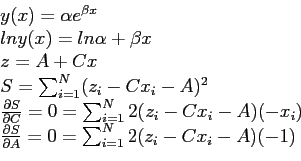
2. Fitting a non-linear curve to the data with least-square method.
   • Use the data in the previous item.
   • We will fit $y(x)=\alpha e^{\beta x}$.
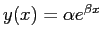   • Repeat each of the steps given in the following solution by hand.
     Solution:
     1. First, we should compute a new table with $z(x)=ln y(x)$

        
        
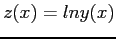
        Then our new data points;
        $$\begin{array}{rr} x & z \hline 0.000 & 0.4055 \\ 0.142 &... ... & -0.1972\\ 0.857 & -0.8164\\ 1.000 & -0.5942\\ \end{array}$$

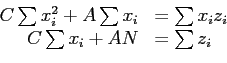
     2. Construct the normal equations (with $A=ln \alpha$ and $C=\beta$)
        $$\begin{array}{l} y(x)=\alpha e^{\beta x}\\ lny(x)=ln\alpha ... ...}{\partial A}=0= \sum_{i=1}^N 2(z_i-Cx_i-A)(-1) \\ \end{array}$$
     3. Dividing each of these equations by $-2$ and expanding the summation, we get the so-called normal equations
        $$\begin{array}{rl} C\sum x_i^2+A\sum x_i & =\sum x_iz_i\\ C\sum x_i+AN & =\sum z_i\\ \end{array}$$

     4. Solve these normal equations to find $A$ and $C$

        
     5. So; we obtained $C=-1.1328$ and $A=0.4466$, we should convert back to the original variables. Convert back to the original variables

        
        we have
        $$z=0.4466-1.1328x, \Rightarrow y=1.563*e^{-1.1328x}$$

     6. Plot $Y$ vs $x$ and $y$ vs $x$ then compare them. For plotting (see Fig. 5.10);

        

        Figure 5.10: plot(x,Y,'o',x,y,'-').

        
   • Compare this least-square polynomial results with the built-in MATLAB functions results in the previous item (item 1), see Fig.5.11.

     

     Figure 5.11: plot(x,Y,'o',x,f,'-',x,y,'+').