Interpolation and Curve Fitting with MATLAB II

1. The MATLAB procedure for polynomial least-squares is polyfit. Study the following example;

   x =(0:0.1:5)'; 					% x from 0 to 5 in steps of 0.1
   y = sin(x); 						% get y values
   p = polyfit(x,y,3); 		% fit a cubic to the data
   f = polyval(p,x); 			% evaluate the cubic on the x data
   plot(x,y,'o',x,f,'-') 	% plot y and its approximation f
   

   Solution:
   

   Figure 5.9: plot(x,y,'o',x,f,'-').

   

   >> x =(0:0.1:5)';
   >> y = sin(x);
   >> p = polyfit(x,y,3)
   p =    0.0919   -0.8728    1.8936   -0.1880
   >> f = polyval(p,x);
   >> plot(x,y,'o',x,f,'-');
   

2. For the given data points;
   $$\begin{array}{rr} x & Y \\ \hline 0.000 & 1.500 \\ 0.142 & ... ...714 & 0.821 \\ 0.857 & 0.442 \\ 1.000 & 0.552 \\ \end{array}$$
   • to which we will fit $y(x)=\alpha e^{\beta x}$
     Hint: First, we should compute a new table with $z(x)=ln y(x)$
     $$\begin{array}{rr} x & z \\ \hline 0.000 & \\ 0.142 & \\ 0.... ...\\ 0.571 & \\ 0.714 & \\ 0.857 & \\ 1.000 & \\ \end{array}$$

   • Construct the normal equations
     Hints: $A=ln \alpha$ and $C=\beta$
   • Solve these normal equations to find $A$ and $C$
   • Convert back to the original variables
   • Plot $Y$ vs $x$ and $y$ vs $x$ then compare them.
   • Soln: $y(x)=1.561e^{-1.132x}$
   Solution:
   

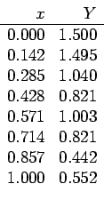
   >> Y=[1.5 1.495 1.04 0.821 1.003 0.821 0.442 0.552]'
   Y =
       1.5000
       1.4950
       1.0400
       0.8210
       1.0030
       0.8210
       0.4420
       0.5520
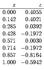
   >> z=log(Y)
   z =
       0.4055
       0.4021
       0.0392
      -0.1972
       0.0030
      -0.1972
      -0.8164
      -0.5942
   

   $$\begin{array}{rr} x & z \\ \hline 0.000 & 0.4055 \\ 0.142 &... ... & -0.1972\\ 0.857 & -0.8164\\ 1.000 & -0.5942\\ \end{array}$$
   $$\begin{array}{l} y(x)=\alpha e^{\beta x}\\ lny(x)=ln\alpha ... ...}{\partial A}=0= \sum_{i=1}^N 2(z_i-Cx_i-A)(-1) \\ \end{array}$$
   Dividing each of these equations by $-2$ and expanding the summation, we get the so-called normal equations
   $$\begin{array}{rl} C\sum x_i^2+A\sum x_i & =\sum x_iz_i\\ C\sum x_i+AN & =\sum z_i\\ \end{array}$$

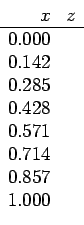
   >> x=[0 0.142 0.285 0.428 0.571 0.714 0.857 1]';
   >> Y=[1.5 1.495 1.04 0.821 1.003 0.821 0.442 0.552]';
   >> z=log(Y);
   >> sum(x'*x)
   ans =    2.8549
   >> sum(x')
   ans =    3.9970
   >> sum(x'*z)
   ans =   -1.4491
   >> sum(z')
   ans =   -0.9553
   >> A=[ 2.8549 3.997; 3.997 8]
   A =
       2.8549    3.9970
       3.9970    8.0000
   >> B=[-1.4491 -0.9553]'
   B =
      -1.4491
      -0.9553
   >> X=uptrbk(A,B)
   X =
      -1.1328
       0.4466
   

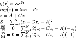
   so; we obtained $C=-1.1328$ and $A=0.4466$, we should convert back to the original variables

   >> exp(0.4466)
   ans =    1.5630
   

   we have
   $$z=0.4466-1.1328x, \Rightarrow y=1.563*e^{-1.1328x}$$
   For plotting;

   >> y=1.5630*exp(-1.1328*x)
   y =
       1.5630
       1.3308
       1.1317
       0.9625
       0.8185
       0.6961
       0.5920
       0.5035
   >> plot(x,Y,'o',x,y,'-')
   

   Figure 5.10: plot(x,Y,'o',x,y,'-').

   
3. Apply the procedure given in the first item by using the data set in the previous item.
   
   • Hints:
     • fit a cubic to the data
     • evaluate the cubic on the x data
   • Plot by $plot(x,Y,'o',x,f,'-')$
   • Compare this least-square polynomial with the function used in the previous item.
   Solution:
   

   >> x=[0 0.142 0.285 0.428 0.571 0.714 0.857 1]';
   >> Y=[1.5 1.495 1.04 0.821 1.003 0.821 0.442 0.552]';
   >> p = polyfit(x,Y,3)
   p =   -0.3476    0.9902   -1.6946    1.5518
   >> f = polyval(p,x)
   f =
       1.5518
       1.3301
       1.1412
       0.9806
       0.8423
       0.7201
       0.6080
       0.4998
   >> plot(x,Y,'o',x,f,'-');
   >> plot(x,Y,'o',x,f,'-',x,y,'+')
   

   Figure 5.11: plot(x,Y,'o',x,f,'-',x,y,'+').