Second Degree Equations

Any second-order or higher-order differential equation can be converted into a system of first-order (linear) equations. For example,

$\displaystyle \frac{d^2y}{dx^2}+A(x)\frac{dy}{dx}+B(x)y(x)=0$
Let's define two new functions for the equation, and :

$\displaystyle y_1(x)=y(x)$ $\displaystyle \$
With this transformation, instead of one 2 $^{nd}$ order equation, two 1 $^{st}$ order equations are formed:

$\displaystyle (1)~~\frac{dy_1}{dx}$ $\displaystyle =$ $\displaystyle y_2(x)$

$\displaystyle (2)~~\frac{dy_2}{dx}$ $\displaystyle =$ $\displaystyle -A(x)y_2-B(x)y_1$

All we need to do to solve higher-order equations, even a system of higher-order initial-value problems, is to reduce them to a system of first-order equations.
Such as: One M-order equation $\rightarrow$ a system with M first-order equations.
Let's take the most general system of differential equations with M unknowns:

$\displaystyle \frac{dy_1}{dx}= f_1(x,y_1,\ldots,y_M)$ $\displaystyle \$

$\displaystyle \vdots ~~~~~~~~~~~~~~$ $\displaystyle ~~~~~~~~~~~ \vdots$ (5.2)

$\displaystyle \frac{dy_M}{dx}= f_M(x,y_1,\ldots,y_M)$ $\displaystyle \$
The next step for solving is to apply the methods (such as; Euler, Runge-Kutta) for the 1 $^{st}$ t order differential equation to these linear system.

We had a set of equations. Two second degree and two first degree differential equations with two unknowns.

$\displaystyle (3)~~~~~~ \frac{d^2x}{dt^2}= -\gamma\left( \sqrt{v_x^2+v_y^2}\right) v_x$	$\displaystyle ~~\&~~$	$\displaystyle (1)~ \frac{dx}{dt}= v_x$
$\displaystyle (4)~ \frac{d^2y}{dt^2}=-g-\gamma\left( \sqrt{v_x^2+v_y^2}\right) v_y$	$\displaystyle ~~\&~~$	$\displaystyle (2)~ \frac{dy}{dt}= v_y$

To solve these two 2 $^{nd}$ degree equations (plus two 1 $^{st}$ degree equations) given above, we first convert them to a system of 4 1 $^{st}$ degree (linear) equations.
To this end, let's define the four unknowns as follows:

Accordingly, the above 2 $^{nd}$ degree system is written as:

$\displaystyle (1)~ \frac{dy_1}{dt}$ $\displaystyle =$ $\displaystyle y_3$

$\displaystyle (2)~ \frac{dy_2}{dt}$ $\displaystyle =$ $\displaystyle y_4$

$\displaystyle (3)~ \frac{dy_3}{dt}$ $\displaystyle =$ $\displaystyle -\gamma \left( \sqrt{y_3^2+y_4^2} \right) y_3$

$\displaystyle (4)~ \frac{dy_4}{dt}$ $\displaystyle =$ $\displaystyle -g-\gamma \left( \sqrt{y_3^2+y_4^2} \right) y_4$
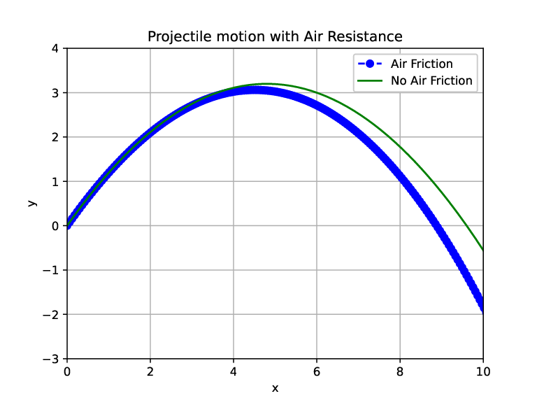
When $\gamma=0$ in this system of equations, we obtain our usual parabolic curve $y=(v_{0y}/v_{0x})x-(g/2v_{0x}^2)x^2$ .

To calculate the effect of air friction, let's take the initial conditions ( $t=0$

) and constants ( $g$

& $\gamma$ ):

**Figure 5.3:** Numerical solution of projectile motion with and without air friction. (Example py-file: airfriction.py)

We had a set of equations. Two second degree and two first degree differential equations with two unknowns.

$\displaystyle (3)~\frac{d^2x}{dt^2}=-G\frac{M}{r^3}x$	$\displaystyle ~~\&~~$	$\displaystyle (1)~ \frac{dx}{dt}= v_x$
$\displaystyle (4)~\frac{d^2y}{dt^2}=-G\frac{M}{r^3}y$	$\displaystyle ~~\&~~$	$\displaystyle (2)~ \frac{dy}{dt}= v_y$

To solve these two 2 $^{nd}$ degree equations (plus two 1 $^{st}$ degree equations) given above, we first convert them to a system of 4 1 $^{st}$ degree (linear) equations.
To this end, let's define the four unknowns as follows:

Accordingly, the above 2 $^{nd}$ degree system is written as:

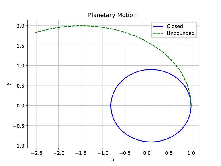
$\displaystyle (1)~ \frac{dy_1}{dt}$ $\displaystyle =$ $\displaystyle y_3$

$\displaystyle (2)~ \frac{dy_2}{dt}$ $\displaystyle =$ $\displaystyle y_4$

$\displaystyle (3)~ \frac{dy_3}{dt}$ $\displaystyle =$ $\displaystyle -\frac{GM}{[y_1^2+y_2^2]^{3/2}}y_1$ (5.3)

$\displaystyle (4)~ \frac{dy_4}{dt}$ $\displaystyle =$ $\displaystyle -\frac{GM}{[y_1^2+y_2^2]^{3/2}}y_2$
For the motion of the planets, we use the astronomical unit system. The Earth-Sun average distance would be in units of astronomical length: $1~au \approx 1.5 \times10^{11}~m$ . The time taken for the Earth to go around the Sun once is 1 year (y) as the unit of time.
Calculated in these units, the product of ,

$\displaystyle GM\approx 40 (au)^3/y^2 % 6.6743e-11 m3/(kg s2)*1.989E30 kg *(365*24*60*60 year)^2/(1.5e11 au)^3= 39,118297342445568$

To calculate the planetary motion, let's take the initial conditions at time t=0 in terms of four unknowns:

$\displaystyle x_0=y_1(t=0)=1.0~au$ $\displaystyle \$

$\displaystyle v_{0x}=y_3(t=0)=0.0$ $\displaystyle \$
Then, also take $v_{0y}=y_4(t=0)=8.0~au/y$ .

**Figure 5.4:** Numerical solution of planetary motion. There can be closed orbits (ellipse), or solutions going to infinity (unbounded, hyperbola) for different velocities. (Example py-file: planetarymotion.py)

$\displaystyle (1)~~\frac{dy_1}{dx}$	$\displaystyle =$	$\displaystyle y_2(x)$
$\displaystyle (2)~~\frac{dy_2}{dx}$	$\displaystyle =$	$\displaystyle -A(x)y_2-B(x)y_1$

$\displaystyle \frac{dy_1}{dx}= f_1(x,y_1,\ldots,y_M)$	$\displaystyle \$
$\displaystyle \vdots ~~~~~~~~~~~~~~$		$\displaystyle ~~~~~~~~~~~ \vdots$	(5.2)
$\displaystyle \frac{dy_M}{dx}= f_M(x,y_1,\ldots,y_M)$	$\displaystyle \$

$\displaystyle (1)~ \frac{dy_1}{dt}$	$\displaystyle =$	$\displaystyle y_3$
$\displaystyle (2)~ \frac{dy_2}{dt}$	$\displaystyle =$	$\displaystyle y_4$
$\displaystyle (3)~ \frac{dy_3}{dt}$	$\displaystyle =$	$\displaystyle -\gamma \left( \sqrt{y_3^2+y_4^2} \right) y_3$
$\displaystyle (4)~ \frac{dy_4}{dt}$	$\displaystyle =$	$\displaystyle -g-\gamma \left( \sqrt{y_3^2+y_4^2} \right) y_4$

$\displaystyle x_0=y_1(t=0)=1.0~au$	$\displaystyle \$
$\displaystyle v_{0x}=y_3(t=0)=0.0$	$\displaystyle \$