Kirchhoff's Rules

Find currents at each loop by using Kirchhoff's Junction & Loop Rules:

3 unkowns, 3 equations

$\begin{indisplay} \begin{array}{r} (R_1+R_2+R_4)i_1-R_2i_2 -R_4i_3=0 \\ -R_2i... ..._3=V_1 \\ -R_4i_1 -R_3i_2+ (R_3+R_4+R_5)i_3=V_2 \\ \end{array}\end{indisplay}$

With the values of $R_1=R_2=1~\Omega$ , $R_3=R_4=R_5=R_6=2~\Omega$ and $V_1=1~V$

. System of linear equations becomes as follows:

$\begin{indisplay} \begin{array}{r} 4i_1-i_2 -2i_3=0 \\ -i_1+ 5i_2-2i_3=1 \\ -2i_1 -2i_2+ 6i_3=5 \\ \end{array}\end{indisplay}$

Example py-file: Kirchhoff's Rules in Gaussian elimination & back substitution. No pivoting. myGEshow_Kirchhoff.py

**Figure 6.2:** Kirchhoff's Rules in Gaussian elimination & back substitution. No pivoting.

Example. Solve the following system of equations using Gaussian elimination.

$\begin{indisplay} \begin{array}{rrrr} &2x_2& &+x_4=0\\ 2x_1 &+2x_2 &+3x_3 &+2... ...3x_2 & & x_4 =-7 \\ 6x_1 &+x_2 &-6x_3 &-5x_4 =6 \\ \end{array}\end{indisplay}$

In addition, obtain the determinant of the coefficient matrix and the $LU$

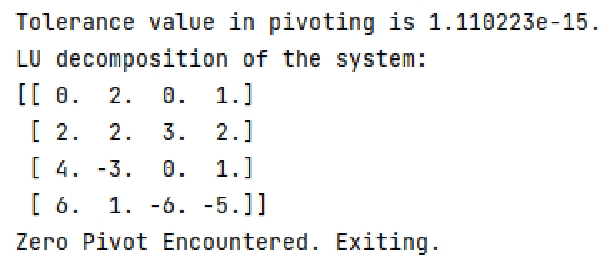
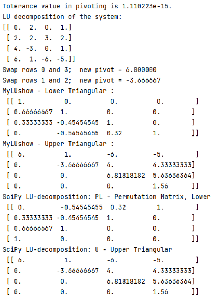
decomposition of this matrix.

1

The augmented coefficient matrix is

$\begin{indisplay} \left[ \begin{array}{rrrrr} 0 & 2 & 0 & 1 &0 \\ 2 & 2 & 3 &... ...4 & -3 & 0 & 1 &-7 \\ 6 & 1 &-6 &-5 &6 \\ \end{array} \right] \end{indisplay}$

2

We cannot permit a zero in the $a_{11}$ position because that element is the pivot in reducing the first column.

3

We could interchange the first row with any of the other rows to avoid a zero divisor, but interchanging the first and fourth rows is our best choice. This gives

$\begin{indisplay} \left[ \begin{array}{rrrrr} 6 & 1 &-6 &-5 &6 \\ 2 & 2 & 3 &... ...4 & -3 & 0 & 1 &-7 \\ 0 & 2 & 0 & 1 &0 \\ \end{array} \right] \end{indisplay}$

$\begin{indisplay} \left[ \begin{array}{rrrrr} 6 & 1 &-6 &-5 &6 \\ 0 &1.6667& ... ...67 & 4 &4.3333&-11 \\ 0 & 2 & 0 & 1 &0 \\ \end{array} \right] \end{indisplay}$

4

We again interchange before reducing the second column, not because we have a zero divisor, but because we want to preserve accuracy. Interchanging the second and third rows puts the element of largest magnitude on the diagonal.

$\begin{indisplay} \left[ \begin{array}{rrrrr} 6 & 1 &-6 &-5 &6 \\ 0 &-3.6667 ... ...6667& 5 &3.6667&-4 \\ 0 & 2 & 0 & 1 &0 \\ \end{array} \right] \end{indisplay}$

5

Now we reduce in the second column

$\begin{indisplay} \left[ \begin{array}{rrrrr} 6 & 1 &-6 &-5 &6 \\ 0 &-3.6667 ... ...001\\ 0 & 0 & 2.1818 & 3.3636 &-5.9999 \\ \end{array} \right] \end{indisplay}$

6

No interchange is indicated in the third column. Reducing, we get

$\begin{indisplay} \left[ \begin{array}{rrrrr} 6 & 1 &-6 &-5 &6 \\ 0 &-3.6667 ... ...&-9.0001\\ 0 & 0 & 0 & 1.5600 &-3.1199 \\ \end{array} \right] \end{indisplay}$

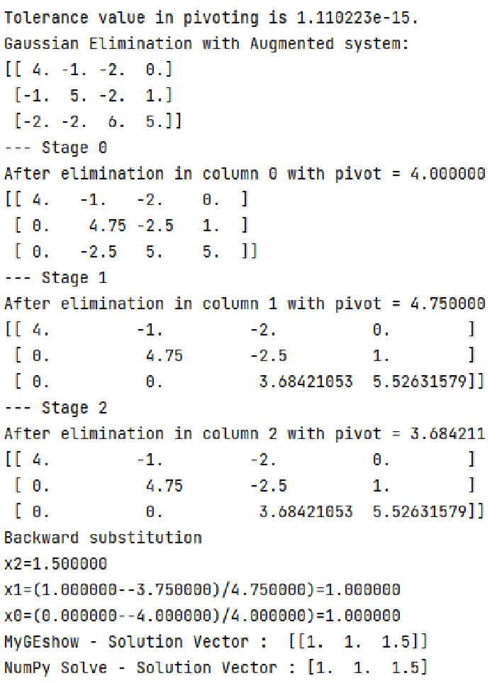
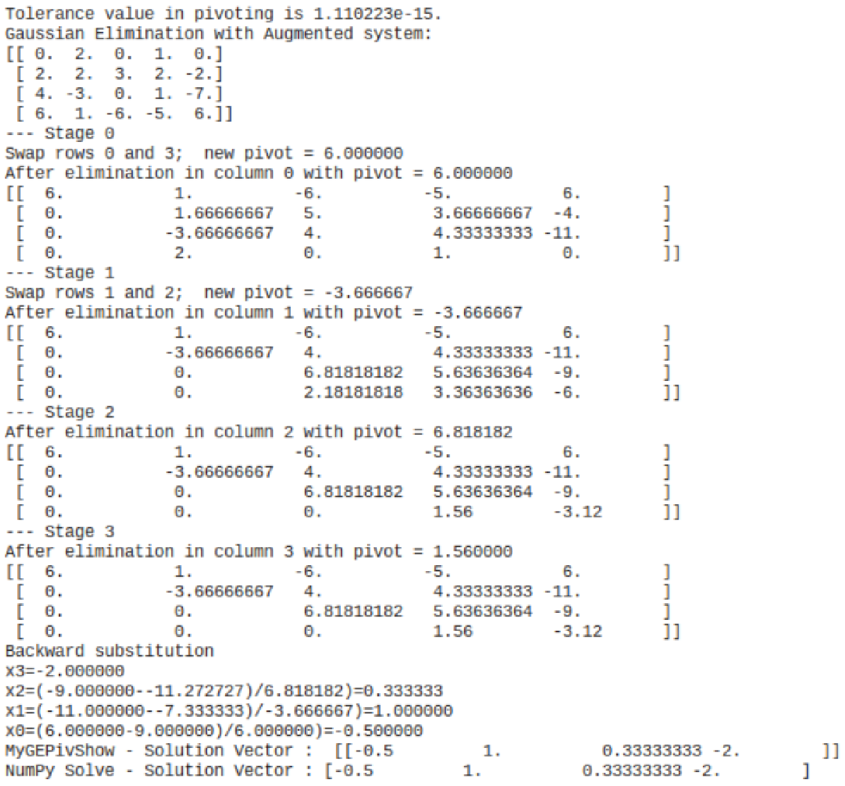
Back-substitution gives

$\displaystyle x_1=-0.50000, x_2=1.0000, x_3=0.33325, x_4=-1.9999.$

The correct (exact) answers are $x_1=-1/2,x_2=1,x_3=1/3,x_4=-2$

. In this calculation we have carried five significant figures and rounded each calculation. Even so, we do not have five-digit accuracy in the answers. The discrepancy is due to round off. Example py-file: Show steps in Gauss elimination and back substitution with pivoting. myGEPivShow.py

**Figure 6.3:** Steps in Gaussian elimination and back substitution with pivoting.

Continue with the previous example.

If we had replaced the zeros below the main diagonal with the ratio of coefficients at each step, the resulting augmented matrix would be

$\begin{indisplay} \left[ \begin{array}{rrrrr} 6 & 1 &-6 &-5 &6 \\ (0.66667) &... ... & (-0.54545) & (0.32) & 1.5600 &-3.1199 \\ \end{array} \right] \end{indisplay}$
This gives a LU decomposition as

$\begin{indisplay} \left[ \begin{array}{rrrrr} 1&0&0&0\\ 0.66667 & 1 & 0 & 0 \... ...54 & 1 &0 \\ 0.0 & -0.54545 & 0.32 & 1 \\ \end{array} \right] \end{indisplay}$

$\begin{indisplay} \left[ \begin{array}{rrrr} 6 & 1 &-6 &-5 \\ 0&-3.6667 & 4 ... ... 0 & 6.8182 &5.6364\\ 0& 0 &0 & 1.5600 \\ \end{array} \right] \end{indisplay}$
It should be noted that the product of these matrices produces a permutation of the original matrix, call it , where

$\begin{indisplay} A'=\left[ \begin{array}{rrrr} 6 & 1 &-6 &-5 \\ 4 & -3 & 0 & 1 \\ 2 & 2 & 3 & 2 \\ 0 & 2 & 0 & 1 \\ \end{array} \right] \end{indisplay}$

The determinant of the original matrix of coefficients can be easily computed according to the formula

$\displaystyle det(A)=(-1)^2*(6)*(-3.6667)*(6.8182)*(1.5600)=-234.0028$
which is close to the exact solution: -234.
The exponent 2 is required, because there were two row interchanges in solving this system.
To summarize
1. The solution to the four equations
2. The determinant of the coefficient matrix
3. A decomposition of the matrix, , which is just the original matrix, , after we have interchanged its rows.
"These" are readily obtained after solving the system by Gaussian elimination method.

Example py-files: LU factorization without pivoting. myLUshow.py LU factorization with pivoting. myLUPivShow.py

Figure 6.4: (a) Without Pivoting (b) With Pivoting.