Next: Nonlinear Data (Curve Fitting) Up: Interpolation and Curve Fitting Previous: The Equation for a Contents
|
|
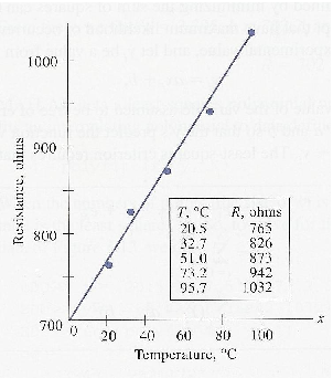
 &
&  , can be obtained from the plot.
& .
, can be obtained from the plot.
& .
|
|
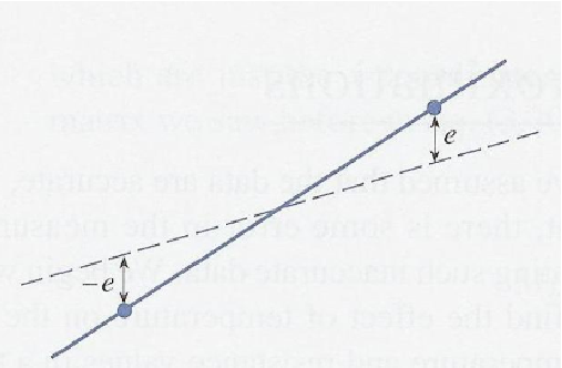
 represent an experimental value, and let
  be a value from the equation

 is a particular value of the variable assumed to be free of error.
& so that the
is a particular value of the variable assumed to be free of error.
& so that the  's predict the function values that correspond to
  -values.

 be a minimum.

 is the number of
  -pairs.
& , so they are the variables of the problem.
, the two partial derivatives will be zero.
-pairs.
& , so they are the variables of the problem.
, the two partial derivatives will be zero.
 and are data points unaffected by our choice our values for and , we have

 and expanding the summation, we get the so-called normal equations

 to
to  .
& .
.
& .


 ,
,  , and
, and

