Least-Squares Polynomials
- Because polynomials can be readily manipulated, fitting such functions to data that do not plot linearly is common.
- We assume the functional relationship
 |
(7.5) |
with errors defined by
- We again use
 to represent the observed or experimental value corresponding to
  , with free of error.
- We minimize the sum of squares;
At the minimum, all the partial derivatives
 vanish.
- Writing the equations for these gives
 equations:
- Dividing each by
 and rearranging gives the normal equations to be solved simultaneously:
 |
(7.6) |
- Putting these equations in matrix form shows the coefficient matrix;
![\begin{indisplay}\left[
\begin{array}{rrrrrl}
N & \sum x_i & \sum x_i^2 & \sum x...
...
\vdots \\
\sum x_i^n Y_i\\
\end{array}\right]
\hspace{-0.5cm}\end{indisplay}](img953.svg) |
|
|
(7.7) |
All the summatins in Eqs. 7.6 and 7.7 run from 1 to  . We will let B stand for the coefficient matrix.
- Equation 7.7 represents a linear system.
- Degrees higher than 4 are used very infrequently. It is often better to fit a series of lower-degree polynomials to subsets of the data.
- Matrix
 of Eq. 7.7 is called the normal matrix for the least-squares problem.
- There is another matrix that corresponds to this, called the design matrix. It is of the form;
 is just the coefficient matrix of Eq. 7.7. It is easy to see that
  , where
  is the column vector of
  -values, gives the right-hand side of Eq. 7.7. We can rewrite Eq. 7.7 in matrix form, as
so it is to find the solution.
- It is illustrated the use of Eq. 7.6 to fit a quadratic to the data of Table 7.7. Figure 7.8 shows a plot of the data.
- The data are actually a perturbation of the relation
 .
.
Table 7.7:
Data to illustrate curve fitting.
Table 7.8:
Figure for the data to illustrate curve fitting.
![\begin{table}
% latex2html id marker 6963
\begin{minipage}[h]{0.6\linewidth}
To ...
...}
\includegraphics[scale=0.5]{images/3.7}
\end{center}
\end{minipage}\end{table}](img959.svg) |
- The equations to be solved are:
The result is
 ,
,
 ,
,
 .
.
- So the least- squares method gives
which we compare to
. Errors in the data cause the equations to differ.
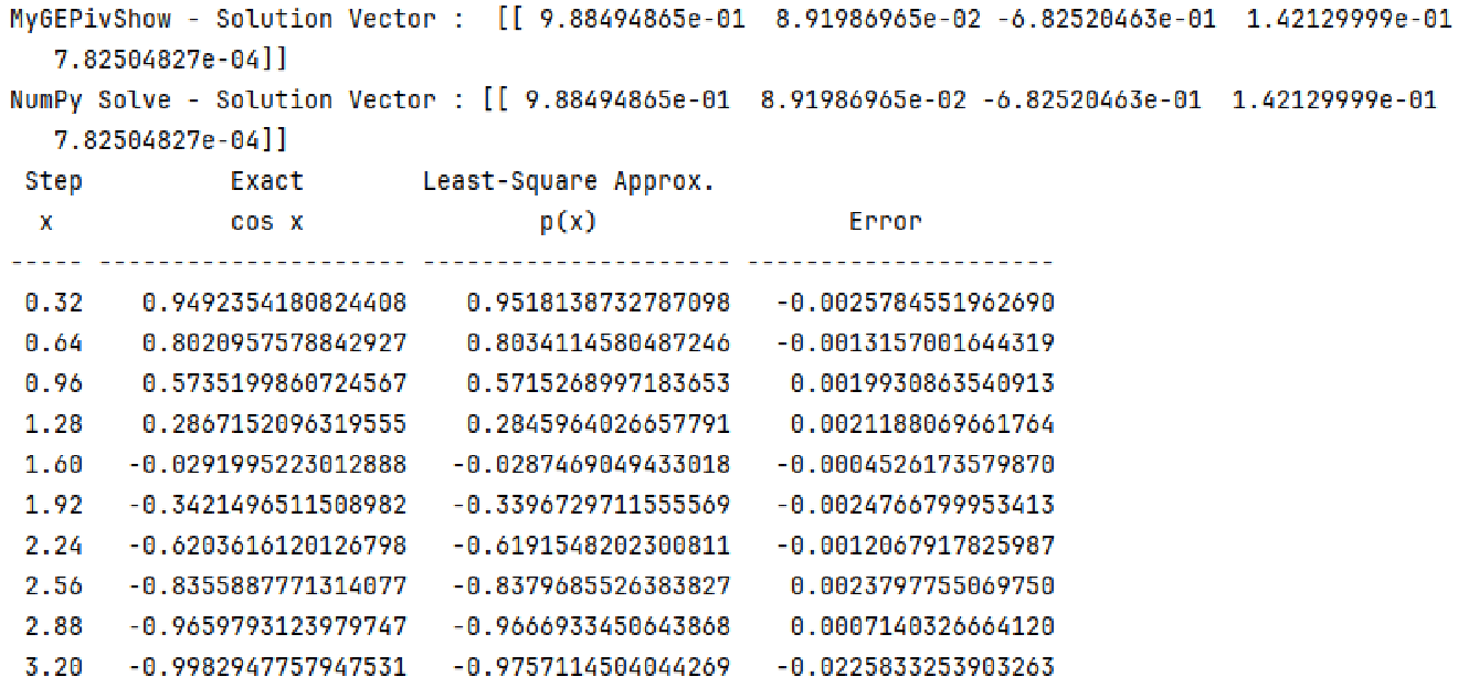
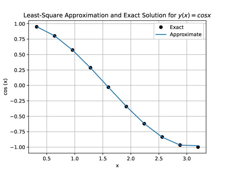
Example py-file: Fitting an 4 order polynomial to
  function in [0,
 ] by Least-Square Approximation. Gaussian elimination & back substitution. Pivoting.
mylsa.py
] by Least-Square Approximation. Gaussian elimination & back substitution. Pivoting.
mylsa.py
Figure 7.10:
Polynomial Least-Square Approximation.
|
|


![\begin{indisplay}
A=\left[
\begin{array}{rrrrr}
1 & 1 & 1 & 1 & 1 \\
x_1 & x_...
...
x_1^n & x_2^n & x_3^n & \ldots & x_N^n\\
\end{array} \right]
\end{indisplay}](img954.svg)